Lotka Volterra Model of Predator-Prey Relationship
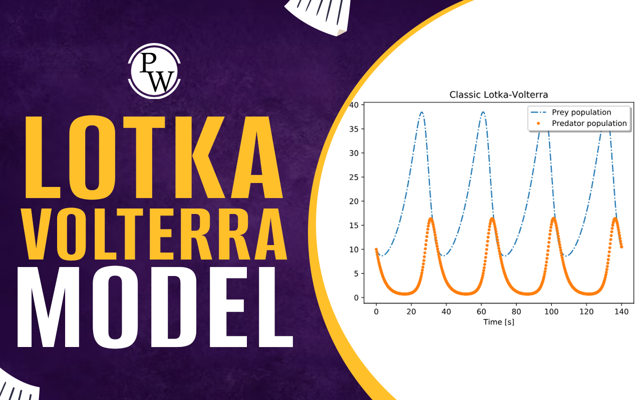
Lotka Volterra: The Lotka Volterra model, also referred to as the predator-prey model, is a well-known mathematical tool for studying the dynamics of interacting biological populations, with a particular emphasis on the interaction between predator and prey species. This model, independently proposed by Alfred J. Lotka and Vito Volterra in 1925 and 1926, has undergone extensive research and served as an important basis for comprehending population dynamics in ecological systems. The Lotka Volterra model is based on two distinct mechanisms: interspecific competition and predator-prey relationships.
Basic Assumptions
It is crucial to comprehend the basic premises of the Lotka Volterra model before delving into the equations and dynamics:
- The model takes interactions between two species—a predator species and a prey species—into account. All other variables are taken to be constant, and it is assumed that these species are the only ones affecting each other's populations.
- Continuous Time: as the model runs in continuous time, population changes are considered a continuous process.
- Unlimited Resources: The model is based on the idea that there are numerous resources available for the prey population to use.
- Instantaneous Response: The model simplifies real-world scenarios by considering that the predator and prey populations react instantly to changes in the other population.
Key Components of the Model
- Prey Population (P): This determines how many herbivores or other small animals there are in the ecosystem as prey.
- Predator Population (Q): This indicates the number of predators in the ecosystem that's main food source is prey.
- Birth Rate (α): The population of prey animals grows naturally in the absence of predators. It determines how quickly the population of prey reproduces in the absence of predators.
- Predation Rate (β): The rate at which predators consume their prey. It measures the number of prey creatures a single predator takes down over a predetermined time frame.
- Efficiency (δ): The efficiency with which prey are transformed into new predators. It demonstrates how many new predators are created for every prey that is consumed.
- Natural Death Rate (γ): The rate at which predators naturally perish when there is no prey available. It gauges how quickly predators perish when there is no food available.
Prey Equation
The first equation describes the change in prey population over time (dP/dt):
dP/dt = αP - βP*Q
The first term, αP, accounts for the exponential growth of the prey population in the absence of predators. As more prey are present, this term drives the population to increase. The second term, βP*Q, represents the predation rate. The more predators (Q) there are and the more prey (P) available, the faster the predators consume them, leading to a decrease in the prey population.
Predator Equation
The second equation details the change in predator population over time (dQ/dt):
dQ/dt = δP*Q - γQ
The first term, δP*Q, represents the growth of the predator population due to the availability of prey. As prey becomes more abundant, predators can reproduce more rapidly. The second term, γQ, accounts for the natural death rate of predators when there is a scarcity of prey.
Lotka Volterra Model of Interspecific Competition
According to theory, we can determine the outcome of interspecific competition between two species using the Lotka Volterra model by looking at the initial population size N, the carrying capacity K, and the competition coefficient. The Lotka Volterra equation for the competition is based on a logistical curve. As a result, the logistical curve equation for the species is as follows:
Species 1: The rate of change of species 1 population (N1) over time (t) is given by:
dN1/dt = r1 * N1 * (K1 - N1 - α12 * N2)
dN1/dt: The rate of change of species 1 population over time.
r1: The intrinsic growth rate of species 1. It represents the maximum rate at which species 1 can reproduce in the absence of competition.
K1: The carrying capacity of species 1. It is the maximum population size that species 1 can sustain given the available resources in the absence of competition.
N1: The population size of species 1 at any given time.
α12: The competition coefficient of species 2 on species 1. It measures the effect of species 2's presence on the growth rate of species 1.
N2: The population size of species 2 at any given time.
The term (K1 - N1 - α12 * N2) represents the available resources for species 1, considering its own carrying capacity, the current population size of species 1, and the effect of competition from species 2.
Species 2: The rate of change of species 2 population (N2) over time (t) is given by:
dN2/dt = r2 * N2 * (K2 - N2 - α21 * N1)
dN2/dt: The rate of change of species 2 population over time.
r2: The intrinsic growth rate of species 2. It represents the maximum rate at which species 2 can reproduce in the absence of competition.
K2: The carrying capacity of species 2. It is the maximum population size that species 2 can sustain given the available resources in the absence of competition.
N2: The population size of species 2 at any given time.
α21: The competition coefficient of species 1 on species 2. It measures the effect of species 1's presence on the growth rate of species 2.
N1: The population size of species 1 at any given time.
The term (K2 - N2 - α21 * N1) represents the available resources for species 2, considering its own carrying capacity, the current population size of species 2, and the effect of competition from species 1.
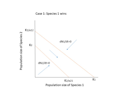
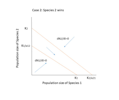
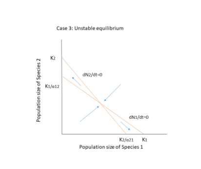
There are three possible outcomes when both species compete.
- The two species will coexist.
- Species 1 goes extinct.
- Extinction of Species 2.
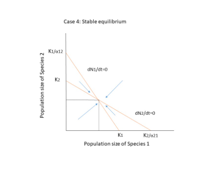
dN1/dt = 0 = dN2/dt
The competing species will have four possible outcomes, as shown in the figure below. Extinction occurs when there is no equilibrium, that is when the diagonals do not cross each other, as in cases 1 and 2. The crossing, on the other hand, results in two points: a stable equilibrium where both species coexist, and an unstable point where even a minor change or disturbance can lead to the extinction of one of the species. In case 4, if the population is slightly declining, they will reach a zone where N1 can increase and N2 can decrease, resulting in species 1 reaching equilibrium on its own at K1.
Limitations
Its limitations include the assumption of constant interaction coefficients, which may not be true in real-world ecosystems. Furthermore, it ignores other ecological factors such as environmental change, spatial distribution, and interactions with other species, all of which can have a significant impact on the dynamics of interspecific competition.