
Biot-Savart Law
Magnetics of Class 12
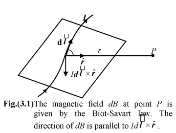
This law tells us about the magnetic field (magnitude and direction) produced by moving charges. The Biot-Savart law is a mathematical description of the magnetic field d
![]() that arises from a current I flowing along an infinitesimal path element d
that arises from a current I flowing along an infinitesimal path element d
![]() called the current element.
called the current element.
The four properties of the magnetic field are as follows.
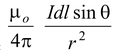
1. The magnetic field grows weaker as we move farther from its source. In particular, the magnitude of the magnetic field d
![]() is inversely proportional to the square of the distance from the current element Id
is inversely proportional to the square of the distance from the current element Id
![]() .
.
2. The larger the electric current, the larger is the magnetic field. In particular, the magnitude of the magnetic field d
![]() is proportional to the current I.
is proportional to the current I.
3. The magnitude of the magnetic field d
![]() is proportional to sin θ, where θ is the angle between the direction of current element Id
is proportional to sin θ, where θ is the angle between the direction of current element Id
![]() and vector
and vector
 that points from the current element to the point in space where dB is evaluated.
4. The direction of the
![]() -is not radially away from its source as the gravitational field and the electric field are from their sources. In fact, the direction of d
-is not radially away from its source as the gravitational field and the electric field are from their sources. In fact, the direction of d
![]() is perpendicular to both Idl and the vector
.
is perpendicular to both Idl and the vector
.
These properties of the magnetic field can be written mathematically as
d
![]() =
=
![]() or d
or d
![]() =
=
![]() (3.1)
(3.1)
|
where
μo = 4π × 10−7 T m/A The direction of the magnetic field element dB as given by Biot Savart law is shown in the figure (3.1).
The direction of
|
|
dB =
 (3.2)
(3.2)
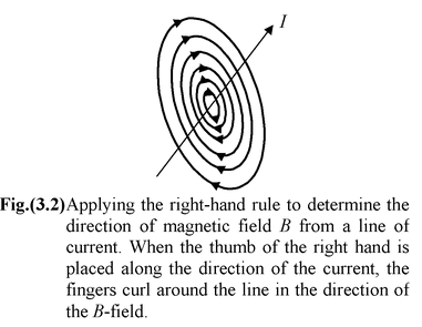
The direction of
![]() can be obtained by applying right hand on Id
can be obtained by applying right hand on Id
![]() ×
×
![]() .
.
For a conducting path of finite length, the total magnetic field B at any given point in space is computed by summing the contributions from each small element of the current along its total path. It can be done by integrating equation (3.2) along the current path made up of dl vectors. In practice one comes across two different cases, each requiring different strategy.
Case 1
The d
![]() contributions from each Id
contributions from each Id
![]() all point in the same direction (or at worst in opposite directions). In this situation one can integrate immediately using the magnitude expression in equation (3.2).
all point in the same direction (or at worst in opposite directions). In this situation one can integrate immediately using the magnitude expression in equation (3.2).
Case 2
The d
![]() contributions from I d
contributions from I d
![]() sources located on different parts of conductor point in different directions. In this case, before integration one must resolve the d
sources located on different parts of conductor point in different directions. In this case, before integration one must resolve the d
![]() contributions into components.
contributions into components.
Case 1 occurs whenever the lines of current and the observation point lie in the same plane.
Example : 3.1
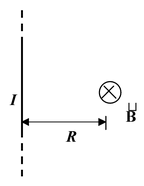
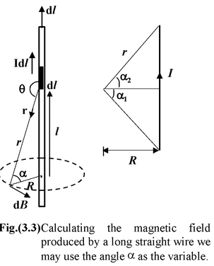
Find the field strength at a distance R from an infinite straight wire that carries a current I.
Solution
Fig. (3.3) shows the infinitesimal contribution to the field, d
![]() from an arbitrary current element. In order to integrate contributions of all the elements, we use the angle α, measure from the perpendicular, as the variable. From the diagram we see that
from an arbitrary current element. In order to integrate contributions of all the elements, we use the angle α, measure from the perpendicular, as the variable. From the diagram we see that
|d
![]() ×
| = dl sin θ
×
| = dl sin θ
= dl sin (π/2 + α)
= dl cos α
Since l = R tan α, we have
dl = R sec2 α dα.
Furthermore,
r = R sec α
|
On substituting these expression into equation (3.1) and integrating we find
B =
=
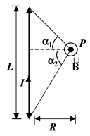
Note that angles on opposite sides of the perpendicular are assigned opposite signs. This ensures that the contributions from either side of the wire add together rather than subtract. For an infinite wire, the limits of integration are -π/2 to +π/2. Thus
B =
|
|
 (sin α1 + sin α2) (3.3)
 (3.4)
(3.4)
Example : 3.2
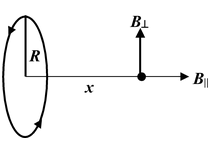
A circular loop of radius a carries a current I. Find the magnetic field along the axis of the loop at a distance x from the centre.
Solution
|
Fig. (3.4) shows the infinitesimal contribution to the field d
|d
|
|
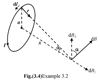
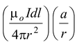
Therefore, the component of dB along the axis is
dB|| = dB sin α =
The total field strength is given by the integral of this expression over all elements. Since the only variable is l, the integral reduces to a sum of length elements.
B|| =
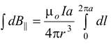
Since ∫ dI = 2πa and r2 = a2 + x2, we may express the result as
B|| =
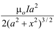 (i) (3.5)
Note that this expression applies only to points on the axis of the loop.
For points far from the loop, that is, when x >> a, (i) becomes,
B|| =
 (3.6)
(3.6)
where pm = I(πa2).
Example: 3.3
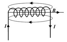
A solenoid of length l and radius a has N turns of wire and carries a current I. Find the field strength at a point along the axis.
Solution
Since the solenoid is a series of closely packed loops. We may use equation (3.5) for the field on the axis of a current carrying loop. The solenoid is divided into current loops of width dy, as in figure (3.5a), each of which contains ndy turns, where n = N/l is the number of turns per unit length. The current within such a loop is (n dy)I. From the diagram we see that
y = a tan θ
from which dy = a sec2θ dθ
Thus, I in equation (3.5) is replaced by
nIdy = nIa sec2θ dθ
After substituting for I and y in equation (3.5) and simplifying, we find
dB =
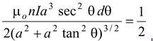 μo nI cos θ dθ
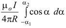
For a finite solenoid, the total field strength is
B = 1/2 μonI ∫ θ2 θ1 cos θ dθ = 1/2μonI (sin θ2 − sin θ1) (3.7)
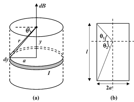
Fig.(3.5) (a) To calculate the field strength along the axis of a solenoid, the solenoid is divided into infinitesimal loops.
(b) The solenoid subtends an angle θ1 and θ2 at the point where we have to obtain the magnetic field.
If the solenoid is infinite long, θ1 = −90° and θ2 = +90°, therefore, the field at the axis of the solenoid is
B = μonI (3.8)
Example : 3.4
(a) What is the magnetic field produced by a point charge q moving at velocity v ?
(b) What is the force between two equal charges moving parallel to each other with the same velocity ?
Solution
(a) The Biot-Savart law refers the magnetic field produced by a current element, Id
![]() .
.
Since I = dq/dt we rewrite
Id
![]() = dq/dt d
= dq/dt d
![]() = dq
= dq
![]() = (dq)
= (dq)
![]()
where
![]() is the velocity of the charge q. From equation (3.1), we infer that the field due to a single charge q moving at velocity v is
is the velocity of the charge q. From equation (3.1), we infer that the field due to a single charge q moving at velocity v is
|
The magnetic field lines are circular, as shown in figure, (3.6 a). (b) In Fig.(3.6 b), the repulsive force between the charges is
FE =
The magnitude of the magnetic force
FB = (qv)
This force is attractive. The net forced between the charge is
F = FE – FB =
Since c2 =
F =
|
|
 , therefore,
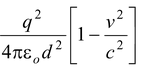
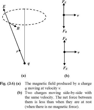
The net force on each of the particles moving with the same velocity is less than that when they are at rest.
Table 3.1 Magnetic field due to different current systems
|
1. A straight wire of finite length
|
B = μoI/4πR(sinα1 + sinα2) |
|
2. An infinitely long straight wire
|
B = μoI/2πR |
|
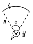
3. An arc of a circle
|
B =
|
|
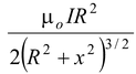
4. On the axis of a Ring
|
B⊥ = 0
B|| =
|
|
5. At the centre of a Ring |
B = μoI /2R |
|
6. On the axis of a solenoid
|
B = μonI = μoN/l I where N is the total number of turns and n is the number of turns per unit length. Assuming that radius of the loop is very small compared to its length. |