

Definite Integral Formula: Definition, Properties, Examples

Before delving into the concept of Definite Integrals , it's essential to review the fundamental notion of integrals in mathematics. Integrals assign numerical values to functions, enabling us to define concepts like displacement, area, volume, and other quantities by connecting infinitesimal data. The mathematical process used to find these integrals is called integration.
There are two primary types of integrals : definite and indefinite integrals. The choice between them depends on whether we specify the boundaries of the integration.
Indefinite Integrals: These are employed when the limits or boundaries of the integrand are not defined. In essence, we find a general antiderivative or a family of functions that satisfy the given integrand.
Definite Integrals: When we specify the lower and upper limits (boundaries) of the independent variable for a function, we use definite integrals. These integrals provide a unique numerical value that represents the accumulated quantity or the net effect of the function within the specified interval.
In the context of definite integrals, various integral formulas and techniques are available to tackle a wide range of mathematical problems. These formulas help us compute the precise numerical values of integrals with specified boundaries, making them a powerful tool in calculus and mathematical analysis.
Definite Integral Definition
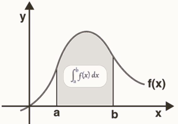
The definite integral of a real-valued function f(x) with respect to a real variable x on an interval [a, b] is expressed as
![]()
Here,
∫ = Integration symbol
a = Lower limit
b = Upper limit
f(x) = Integrand
dx = Integrating agent
Thus, ∫ab f(x) dx is read as the definite integral of f(x) with respect to dx from a to b.
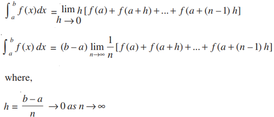
Definite Integral as Limit of Sum
The definite integral of any function can be expressed either as the limit of a sum or if there exists an antiderivative F for the interval [a, b], then the definite integral of the function is the difference of the values at points a and b. Let us discuss definite integrals as a limit of a sum. Consider a continuous function f in x defined in the closed interval [a, b]. Assuming that f(x) > 0, the following graph depicts f in x.
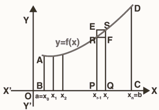
The integral of a function f(x) can indeed be visualized as the area under the curve y = f(x) within a given interval [a, b]. To understand this concept better, we can divide the interval [a, b] into smaller subintervals as described:
The entire region between [a, b] is divided into n equal subintervals, each with a width of h.
The subintervals are represented as [x 0 , x 1 ], [x 1 , x 2 ], ..., [x r-1 , x r ], [x n-1 , x n ], where x 0 = a, x 1 = a + h, x 2 = a + 2h, ..., x r = a + rh, and x n = b = a + nh.
The number of subintervals, n, can be calculated as n = (b – a)/h.
As n approaches infinity (i.e., n → ∞), the subintervals become infinitesimally small, and the width h approaches zero.
Now, let's examine the relationships between the areas of specific regions and intervals within this context:
Area of rectangle PQFR < Area of the region PQSRP < Area of rectangle PQSE
This inequality (1) represents the comparison of areas within the region bounded by the curve y = f(x), where PQFR represents the area under the curve, PQSRP represents the area within the curve, and PQSE represents the area above the curve.
Since h → 0, therefore x r – x r-1 → 0.
This statement emphasizes that as the subintervals become infinitesimally small (h → 0), the difference between consecutive x-values (x r – x r-1 ) also tends to zero. This is a crucial concept in the limit definition of the integral.
The following sums can be established as
The "following sums" likely refer to the limits and sums that are used to define the integral as the limit of a Riemann sum. In this context, as n approaches infinity, you can express the definite integral of f(x) over the interval [a, b] as the limit of a sum:
∫[a, b] f(x) dx = lim (n → ∞) Σ[f(xi) * Δxi]
Here, xi represents points within each subinterval, f(xi) is the value of the function at xi, Δxi is the width of the subinterval (which approaches zero as n → ∞), and the sum Σ is taken over all subintervals.
These relationships and limits are fundamental in understanding how the integral of a function represents the area under the curve and how it is calculated as the limit of a sum as the number of subintervals approaches infinity and their widths approach zero.
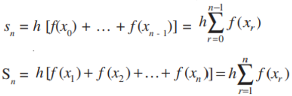
Expanding on the first inequality, let's focus on an arbitrary subinterval [xr-1, xr], where r can take on values from 1 to n. In this context, we can assert that the sum of areas within these subintervals, represented as "sn," is less than the total area of the region ABCD, which is bounded by the curve y = f(x), and this, in turn, is less than the sum "Sn" of areas of rectangles.
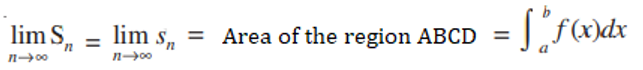
As n approaches infinity, the subintervals become extremely narrow, essentially becoming infinitesimally small strips. In this limit, we can assume that the limiting values of sn and Sn are equal. This common limiting value provides us with the area under the curve, i.e., it represents the integral of the function:
∫[a, b] f(x) dx = lim (n → ∞) sn = lim (n → ∞) Sn
In this way, as the number of subintervals increases without bound and their widths approach zero, we obtain the precise area under the curve y = f(x), which corresponds to the definite integral of the function over the interval [a, b].
Indeed, from this perspective, we can conclude that the area under the curve, represented by the definite integral, is also the limit of the area that lies between the rectangles below and above the curve.
In other words, as we let the number of subintervals approach infinity and the width of each subinterval approach zero, the area between the rectangles that approximate the region under the curve becomes an increasingly accurate representation of the actual area under the curve. This common limiting value serves as a precise measure of the area bounded by the curve, and it is captured by the definite integral of the function over the specified interval.
This is known as the definition of definite integral as the limit of sum.
Also Check – Line and Angles Formula
Definite Integral Properties
Below is the list of some essential properties These will help evaluate the definite integrals more efficiently.
- ∫ a b f(x) dx = ∫ a b f(t) d(t)
- ∫ a b f(x) dx = – ∫ b a f(x) dx
- ∫ a a f(x) dx = 0
- ∫ a b f(x) dx = ∫ a c f(x) dx + ∫ c b f(x) dx
- ∫ a b f(x) dx = ∫ a b f(a + b – x) dx
- ∫ 0 a f(x) dx = f(a – x) dx
Also Check – Introduction to Graph Formula
Definite Integral by Parts
Below are the formulas to find the definite integral of a function by splitting it into parts.
- ∫ 0 2a f (x) dx = ∫ 0 a f (x) dx + ∫ 0 a f (2a – x) dx
- ∫ 0 2a f (x) dx = 2 ∫ 0 a f (x) dx … if f(2a – x) = f (x).
- ∫ 0 2a f (x) dx = 0 … if f (2a – x) = – f(x)
- ∫-a a f(x) dx = 2 ∫ 0 a f(x) dx … if f(- x) = f(x) or it is an even function
- ∫ -a a f(x) dx = 0 … if f(- x) = – f(x) or it is an odd function
Also Check – Factorization Formula
Definite Integral Examples
Example 1:
To find the value of ∫ 2 3 x 2 dx, we'll follow these steps:
Let I = ∫ 2 3 x 2 dx
Now, ∫x 2 dx = (x 3 )/3
Now, I = ∫ 2 3 x 2 dx = [(x 3 )/3] 2 3
= (3 3 )/3 – (2 3 )/3
= (27/3) – (8/3)
= (27 – 8)/3
= 19/3
Therefore, ∫ 2 3 x 2 dx = 19/3
Example 2:
To calculate ∫ 0 π/4 sin 2x dx, we'll proceed as follows:
Let I = ∫ 0 π/4 sin 2x dx
Now, ∫ sin 2x dx = -(½) cos 2x
I = ∫ 0 π/4 sin 2x dx
= [-(½) cos 2x] 0 π/4
= -(½) cos 2(π/4) – {-(½) cos 2(0)}
= -(½) cos π/2 + (½) cos 0
= -(½) (0) + (½)
= 1/2
Therefore, ∫ 0 π/4 sin 2x dx = 1/2
Definite Integral Formula FAQs
Q1. What is a definite integral?
Q2. What is the formula for the definite integral?
Q3. What is a definite integral used for?
Q4. Can a definite integral be negative?
Q5. Do definite integrals have a constant term 'C'?