

Lagrange Interpolation Formula: Definition, Properties, Uses

Lagrange Interpolation is a mathematical technique used to approximate a function within a certain range using a polynomial that passes through a given set of data points. It is named after the Italian-French mathematician Joseph-Louis Lagrange. This interpolation method is particularly useful when you have a discrete set of data points and want to estimate values between those data points.
Lagrange Interpolation is a valuable tool in numerical analysis and approximation theory. It allows you to create a smooth polynomial representation of a function based on limited data, making it useful in various fields such as physics, engineering, computer graphics, and more. However, it's worth noting that higher-degree Lagrange Polynomials can exhibit oscillations between data points, and in such cases, alternative interpolation methods like cubic splines may be preferred.
What is Lagrange Interpolation?
Lagrange Interpolation is a mathematical technique used to estimate the value of a function at any specified point within a certain range, even when the function itself is not explicitly known. This method relies on using known data points from the function to interpolate values at other points.
Lagrange Interpolation allows us to approximate the value of a function at any desired point, even if we don't have the explicit formula for that function. It involves using known data points from the function to make these estimates. Suppose we have a function, y = f(x), where different values of y result from substituting different values of x. If we are provided with two specific points (x1, y1) and (x2, y2) on the curve, we can use the Lagrange Interpolation Formula to calculate the value of y at a constant x = a. This formula helps us construct a polynomial that fits the known data points and can be used to find the function's values at other points, including x = a.
Lagrange Interpolation Formula
The fundamental concept of polynomial interpolation. Given a set of real values x 1 , x 2 , x 3 , …, x n and corresponding y 1 , y 2 , y 3 , …, y n you can find a polynomial P(x) with real coefficients such that it satisfies the conditions:
P(x i ) = yi, ∀ i = {1, 2, 3, …, n} meaning the polynomial passes through all the given data points.
The degree of the polynomial P must be less than n, which means it is a polynomial of degree less than the number of data points.
This interpolation problem seeks to find a polynomial that smoothly connects the data points and can be used to estimate the function's values between those points. Polynomial interpolation is widely used in various fields of mathematics and science for data analysis, curve fitting, and approximation.
The specific method you would use to find the polynomial P is often the Lagrange Interpolation method, which constructs a polynomial that passes through the given data points. Other interpolation techniques, such as Newton's divided differences or cubic splines, can also be employed, depending on the context and desired properties of the interpolating polynomial.
Lagrange Interpolation Formula for n th Order
The Lagrange Interpolation formula for nth degree polynomial is given below:
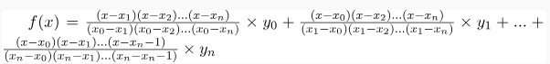
Lagrange Interpolation Formula for the n th order is,
Lagrange First Order Interpolation Formula
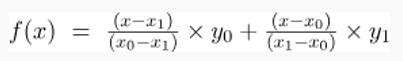
If the Degree of the polynomial is 1 then it is called the First Order Polynomial. The Lagrange Interpolation Formula for 1st order polynomials is,
Lagrange Second Order Interpolation Formula
If the Degree of the polynomial is 2 then it is called Second Order Polynomial. The Lagrange Interpolation Formula for 2nd order polynomials is,

Proof of Lagrange Theorem
Let’s consider a nth-degree polynomial of the given form,
f(x) = A 0 (x – x 1 )(x – x 2 )(x – x 3 )…(x – x n ) + A 1 (x – x 1 )(x – x 2 )(x – x 3 )…(x – x n ) + … + A (n-1 )(x – x 1 )(x – x 2 )(x – x 3 )…(x – x n )
Substitute observations xi to get Ai
Put x = x 0 then we get A 0
f(x 0 ) = y 0 = A 0 (x 0 – x 1 )(x 0 – x 2 )(x 0 – x 3 )…(x 0 – x n )
A 0 = y 0 /(x 0 – x 1 )(x 0 – x 2 )(x 0 – x 3 )…(x 0 – x n )
By substituting x = x1 we get A1
f(x 1 ) = y 1 = A 1 (x 1 – x 0 )(x 1 – x 2 )(x 1 – x 3 )…(x 1 – x n )
A 1 = y 1 /(x 1 – x 0 )(x 1 – x 2 )(x 1 – x 3 )…(x 1 – x n )
Similarly, by substituting x = x n we get A n
f(x n ) = y n = A n (x n – x 0 )(x n – x 1 )(x n – x 2 )…(x n – x n-1 )
A n = y n /(x n – x 0 )(x n – x 1 )(x n – x 2 )…(x n – x n-1 )
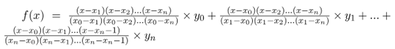
If we substitute all values of Ai in function f(x) where i = 1, 2, 3, …n then we get Lagrange Interpolation Formula as,
Properties of Lagrange Interpolation Formula
The properties you've mentioned pertain to the Lagrange Interpolation Formula. Let's discuss these properties in detail:
- Estimating Function Values: The Lagrange Interpolation Formula is indeed used to estimate the value of a function at any specified point, even when the explicit function is not known. It's a valuable tool for interpolation, allowing you to approximate the function's values between known data points.
- Non-Uniform Data Points: Lagrange Interpolation is not limited to evenly spaced data points. It can handle data points that are irregularly spaced. This flexibility is essential because in many practical applications, data points are not evenly distributed along the independent variable.
- Numerical Analysis: Lagrange Interpolation is widely used in numerical analysis. It helps find approximate values of a function at points within a given range based on known data points. This is crucial for solving real-world problems in various fields, including science, engineering, and computer science.
In summary, the Lagrange Interpolation Formula is a versatile tool for estimating function values between given data points, regardless of whether the data points are evenly spaced or not. Its applications extend to numerical analysis and various fields where data approximation is necessary for making predictions or solving problems.
Uses of Lagrange Interpolation Formula
The Lagrange Interpolation Formula is a versatile mathematical tool with several practical applications. Let's discuss the mentioned uses and some additional applications:
- Function Approximation: As previously mentioned, the primary use of the Lagrange Interpolation Formula is to estimate the value of the dependent variable at a specific independent variable when the explicit function is not given. This is particularly useful in numerical analysis and engineering for data interpolation.
- Image Scaling: Lagrange Interpolation is used in image processing for resizing or scaling images. It helps in generating additional pixels to make the image larger or reducing the number of pixels to make the image smaller while maintaining smooth transitions.
- AI Modeling: Lagrange Interpolation can be used in artificial intelligence modeling for data smoothing, feature engineering, and approximating functions within machine learning algorithms. It plays a role in generating smooth curves or surfaces to fit data points.
- Natural Language Processing (NLP): While not a direct application, interpolation methods, including Lagrange, may be used in NLP and text processing for various tasks like text generation and language modeling. It can help create continuous, coherent text based on existing data.
- Signal Processing: In signal processing, Lagrange Interpolation can be employed to estimate data values at non-uniformly sampled points, making it useful for tasks such as audio signal reconstruction.
- Computer Graphics: Lagrange Interpolation plays a role in computer graphics for tasks like curve and surface modeling, which is essential in 2D and 3D rendering.
- Financial Modeling: In finance, Lagrange Interpolation can be used to estimate intermediate values for various financial parameters, which is valuable for option pricing and risk analysis.
- Scientific Data Analysis: Lagrange Interpolation is used in various scientific fields to approximate missing data points or to generate smooth curves when working with experimental data.
- GPS and Navigation: In navigation systems, Lagrange Interpolation can be used to estimate a location between known GPS data points, aiding in real-time tracking and route planning.
- Astronomy: Astronomers use interpolation methods, including Lagrange Interpolation, for estimating the positions of celestial bodies at specific times.
These are just a few examples of the diverse applications of the Lagrange Interpolation Formula. It is a valuable tool in mathematics, science, engineering, and technology, where data points need to be connected or where values need to be estimated between known data points.
| Related Links | |
| Difference Quotient Formula | Probability |
| Effect Size Formula | Consecutive Integers Formula |
Lagrange Interpolation Formula FAQs
Q1. What is the Lagrange Interpolation Formula?
Q2. When is the Lagrange Interpolation Formula used?
Q3. How is the Lagrange Polynomial constructed?
Q4. What are the properties of the Lagrange Interpolation Formula?
Q5. What are the limitations of Lagrange Interpolation?