

Linear Inequalities Formula: Rules, Graph, Examples

In the Linear Inequalities formula inequality arises when a comparison is made between two mathematical expressions or two numbers, and they are found not to be equal. Inequality can take various forms, including numerical inequalities and algebraic inequalities, or even a combination of both. Linear inequalities specifically involve at least one linear algebraic expression, typically a polynomial of degree 1, being compared with another algebraic expression of degree less than or equal to 1. There exist several methods to represent and work with different types of linear inequalities.
In this article, we will delve into the topic of linear inequalities, exploring concepts such as solving linear inequalities and graphing linear inequalities to gain a comprehensive understanding of this mathematical concept.
What Are Linear Inequalities Formula?
Linear inequalities can be described as mathematical expressions in which two linear expressions are contrasted using inequality symbols. There are five symbols commonly employed to denote linear inequalities, and they are as follows:
| Symbol Name | Symbol | Example |
| Not equal | ≠ | x ≠ 3 |
| Less than | (<) | x + 7 < √2 |
| Greater than | (>) | 1 + 10x > 2 + 16x |
| Less than or equal to | (≤) | y ≤ 4 |
| Greater than or equal to | (≥) | -3 - √3x ≥ 10 |
It's important to understand the distinctions between the inequality symbols. When we have p < q, it signifies that p is a number strictly less than q. On the other hand, p ≤ q indicates that p is a number that can be either strictly less than q or equal to q. The same logic applies to the other two inequalities: > (greater than) and ≥ (greater than or equal to).
Also Check - Rational Numbers Formula
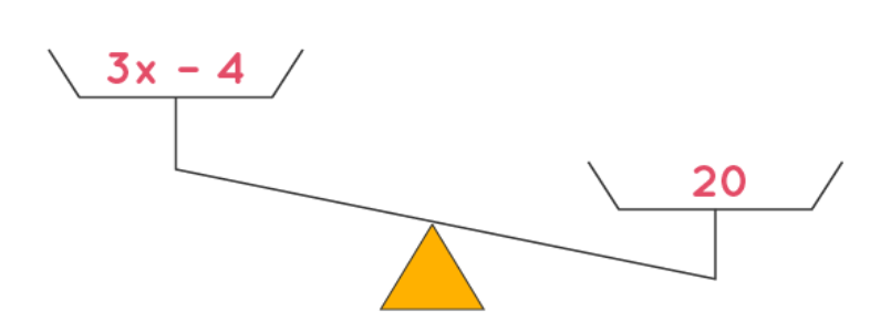
Now, let's consider a linear inequality like 3x - 4 < 20. In this case, the left-hand side (LHS), which is 3x - 4, is indeed smaller than the right-hand side (RHS), which is 20. We can visually represent this inequality as if we were balancing weights on a scale:
Rules of Linear Inequalities Formula
There are four fundamental operations involved in working with linear inequalities: addition, subtraction, multiplication, and division. When two linear inequalities have the same solution, they are termed equivalent inequalities. These rules apply to inequalities involving "less than or equal to" (≤) and "greater than or equal to" (≥) as well. Before delving into the process of solving linear inequalities, it's essential to understand some crucial rules governing inequalities for each of these operations.
Also Check - Linear Equation Formula
- Addition Rule for Linear Inequalities:
The addition rule for linear inequalities states that adding the same number to both sides of an inequality results in an equivalent inequality, with the inequality symbol remaining unchanged.
For instance, if x > y, then x + a > y + a. Similarly, if x < y, then x + a < y + a.
- Subtraction Rule for Linear Inequalities:
The subtraction rule for linear inequalities dictates that subtracting the same number from both sides of an inequality produces an equivalent inequality, with the inequality symbol staying the same.
For example, if x > y, then x − a > y − a. Likewise, if x < y, then x − a < y − a.
Also Check - Quadrilaterals Formula
- Multiplication Rule for Linear Inequalities:
The multiplication rule for linear inequalities states that multiplying both sides of an inequality by a positive number results in an equivalent inequality, with the inequality symbol remaining unaltered.
For instance, if x > y and a > 0, then x × a > y × a. Conversely, if x < y and a > 0, then x × a < y × a. Note that "×" represents the multiplication symbol.
However, when multiplying both sides of an inequality by a negative number, the inequality direction must be reversed to maintain equivalence:
For instance, if x > y and a < 0, then x × a < y × a. Similarly, if x < y and a < 0, then x × a > y × a.
- Division Rule for Linear Inequalities:
The division rule for linear inequalities asserts that dividing both sides of an inequality by a positive number results in an equivalent inequality, with the inequality symbol remaining unaltered.
For instance, if x > y and a > 0, then (x/a) > (y/a). Conversely, if x < y and a > 0, then (x/a) < (y/a).However, when dividing both sides of an inequality by a negative number, the inequality direction must be reversed to maintain equivalence:
For instance, if x > y and a < 0, then (x/a) < (y/a). Similarly, if x < y and a < 0, then (x/a) > (y/a).
Solving System Of Linear Inequalities
Solving linear inequalities with one variable in multiple steps follows a similar approach to solving multi-step linear equations. The primary objective is to isolate the variable while adhering to the rules of inequalities. It is crucial to remember that when multiplying or dividing by negative numbers, the inequality sign must be reversed, as dictated by the inequality rules.
Step 1: Begin by simplifying the inequality on both sides, following the rules of inequalities.
Step 2: After obtaining the value, if the inequality is strict (not inclusive of equal to), the solution for variable 'x' will either be strictly less than or strictly greater than the value as defined in the question. If the inequality is not strict, the solution for 'x' will include values less than or equal to or greater than or equal to the specified value.
Let's illustrate this concept with an example:
Consider the inequality: 2x + 3 > 7
To solve this linear inequality, we follow these steps:
2x > 7 - 3 ⇒ 2x > 4 ⇒ x > 2
The solution to this inequality consists of all values of 'x' that satisfy x > 2, which means all real numbers greater than 2.
Now, let's apply this approach to a linear inequality with variables on both sides:
Example: 3x - 15 > 2x + 11
We proceed as follows:
-15 - 11 > 2x - 3x ⇒ -26 > -x ⇒ x > 26
In this case, the solution for 'x' is all real numbers greater than 26, as indicated by the inequality x > 26.
Solving System of Linear Inequalities by Graphing
A system of linear inequalities with two variables is typically represented in the form of ax + by > c or ax + by ≤ c, where 'a,' 'b,' and 'c' are constants. The direction of the inequality signs (>, <, ≥, ≤) can vary based on the specific set of inequalities provided. To solve a system of two-variable linear inequalities, it is necessary to have at least two inequalities.
Let's proceed to solve a system of linear inequalities in two variables with an example:
Example: Consider the following system of inequalities:
2y - x > 1 and y - 2x < -1
To begin, we'll graph the given inequalities using the following steps:
Replace the inequality signs with equal signs (=), resulting in 2y - x = 1 and y - 2x = -1. Since the inequalities are strict, we draw dotted lines on the graph.
Check if the origin (0, 0) satisfies the given linear inequalities. If it does, shade the region on one side of the line that includes the origin. If the origin does not satisfy the linear inequality, shade the region on one side of the line that does not include the origin.
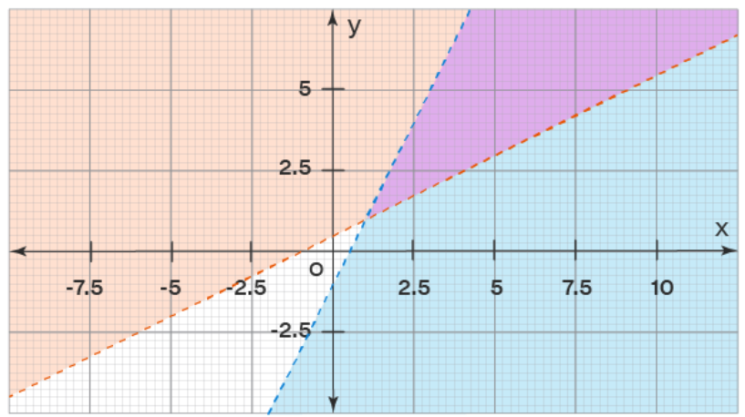
For 2y - x > 1, substituting (0, 0) yields: 2 × 0 - 0 > 1 ⇒ 0 > 1, which is not true. Therefore, shade the side of the line 2y - x = 1 that does not include the origin.
Similarly, for y - 2x < -1, substituting (0, 0) gives: 0 - 2 × 0 < -1 ⇒ 0 < -1, which is not true. Thus, shade the side of the line y - 2x = -1 that does not include the origin.
The common shaded region on the graph represents the feasible region and constitutes the solution to the system of linear inequalities. If there is no common shaded region, it indicates that a solution does not exist. In the provided graph, the violet-colored region signifies the solution to the given system of linear inequalities.
Graphing Linear Inequalities
Linear inequalities involving a single variable are typically represented on a number line, as the result provides the solution for just one variable. Consequently, the graphical representation of linear inequalities with one variable is exclusively done using a number line. In contrast, linear inequalities involving two variables are graphed on a two-dimensional coordinate system with x and y axes because the solution pertains to two variables. Therefore, the process of graphing two-variable linear inequalities is carried out using a graph or a coordinate plane.
Graphing Linear Inequalities - One Variable
Let's examine the following example:
Example 1: Consider the inequality 4x > -3x + 21.
The solution to this inequality is straightforward:
4x + 3x > 21 ⇒ 7x > 21 ⇒ x > 3
We can represent this solution on a number line as follows:
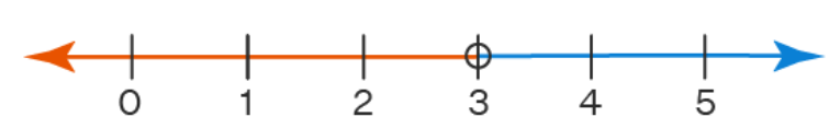
[Number Line Graphic]
In this case, any point located on the blue portion of the number line satisfies the inequality. It's worth noting that a hollow dot is placed at point 3 to indicate that 3 is not part of the solution set, as the given inequality is strict.
Now, let's explore another example of a linear inequality:
Example 2: Consider the inequality 3x + 1 ≤ 7.
We proceed with the solution:
3x ≤ 7 - 1 ⇒ 3x ≤ 6 ⇒ x ≤ 2
To represent this solution set on a number line, we highlight the section of the number line to the left of 2:
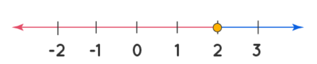
[Number Line Graphic]
Here, any number situated on the red section of the number line satisfies the inequality, making it a part of the solution set. Additionally, a solid dot is placed precisely at point 2 to indicate that 2 is indeed included in the solution set.
Linear Inequalities Formula FAQs
Define the term Linear Inequalities formula.
Give an example of Linear Inequalities.
Give a real life application of a linear equation?
Define the Symbols used for linear inequalities.