

Matrix Multiplication Formula - Definition and Conditions

In the realm of linear algebra, matrices hold a significant position when it comes to addressing various mathematical concepts. A matrix is essentially a structured arrangement of numbers, symbols, or expressions organized in rows and columns. This mathematical construct enables us to execute a multitude of operations, including but not limited to addition, subtraction, and multiplication. Within this article, we will delve into the intricate process of matrix multiplication, discussing its algorithm and formula. We will also provide detailed examples showcasing the multiplication of 2×2 and 3×3 matrices, offering a comprehensive understanding of this fundamental mathematical operation.
Matrix Multiplication Definition
Matrix multiplication, also referred to as matrix product, is an operation that combines two matrices to yield a single matrix. This operation is categorized as a binary operation.
When considering two matrices, A and B, their product is symbolically represented as follows:
X = AB
In essence, matrix multiplication can be thought of as the dot product of the two matrices.
Scalar Multiplication of Matrices:
Multiplying a matrix by a scalar value is a straightforward operation known as scalar multiplication.
As we know, a matrix is an organized collection of numbers arranged in rows and columns. When you multiply a matrix by a scalar value, it is termed scalar multiplication. Alternatively, you can multiply one matrix by another matrix. To illustrate this concept, let's examine the following example.
Mathematically, we can define the multiplication of a matrix by a scalar as follows:
If A = [aij]m × n represents a matrix and k is a scalar, then kA is a resulting matrix obtained by multiplying each element of A by the scalar k.
In simpler terms, kA = k [aij]m × n = [k (aij)]m × n. In this context, the (i, j)th element of kA is equal to k times aij for all possible values of i and j .
Example:
Solution: We have
we have to multiply the given element of the matrix A by 4.
this is the required answer.
Also Check - Arithmetic Progression Formula
Matrix multiplication Condition
In order to execute the multiplication of two matrices, it is imperative that the number of columns in the first matrix matches the number of rows in the second matrix. Consequently, the resulting matrix product will inherit the number of rows from the first matrix and the number of columns from the second matrix. This arrangement defines the order or dimensions of the resulting matrix, known as the matrix multiplication order.
Multiplying matrices involves performing a series of operations where the entries of one matrix are combined with the entries of another matrix to produce a new matrix. To multiply two matrices A and B, follow these steps:
Check Compatibility:
Ensure that the number of columns in matrix A matches the number of rows in matrix B. In other words, matrix A must be of size m x n, and matrix B must be of size n x p to be compatible for multiplication.
Initialize the Resultant Matrix:
Create an empty matrix, often denoted as C, with dimensions m x p, where m is the number of rows from matrix A, and p is the number of columns from matrix B.
Calculate the Entries of the Resultant Matrix:
For each element C[i][j] in the resultant matrix C, calculate it using the dot product of the corresponding row from matrix A and column from matrix B. The formula for the element C[i][j] is:
C[i][j] = A[i][1]*B[1][j] + A[i][2]*B[2][j] + ... + A[i][n]*B[n][j]
Perform the Dot Products:
Calculate the dot product of row i from matrix A and column j from matrix B to get the value for C[i][j]. This involves multiplying corresponding elements from both matrices and summing them up.
Repeat for All Entries:
Repeat the dot product calculation for all elements in the resultant matrix C, filling in each element's value.
Also Check - Data Handling Class 8 Formula
Matrix Multiplication Formula
For a better picture of the Matrix Multiplication Formula let's take an example to understand this formula.
Considering two matrices A and B such that,
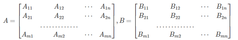
Matrix C = AB is denoted by
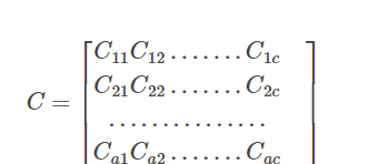
An element in matrix C where C is the multiplication of Matrix A X B.
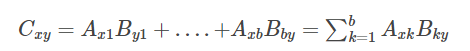
For x = 1…… a and y= 1…….c
Algorithm for Matrix Multiplication
Matrix multiplication is a critical operation with wide-ranging applications, leading to the development of various algorithms over the years. There are four primary types of matrix multiplication algorithms:
Iterative Algorithm: This approach involves systematically multiplying corresponding elements of matrices and summing them up. It's commonly used for smaller matrices like 2x2, 3x3, and 4x4.
Divide and Conquer Algorithm: This method breaks down the matrix multiplication problem into smaller sub-problems, multiplies them recursively, and combines the results. It's useful for larger matrices and reduces the overall computational complexity.
Sub-cubic Algorithms: These advanced algorithms aim to achieve matrix multiplication with a computational complexity lower than the traditional cubic complexity. They are designed to improve efficiency for large matrices.
Parallel and Distributed Algorithms: With the rise of parallel computing and distributed systems, algorithms have been developed to perform matrix multiplication efficiently in parallel or on distributed computing architectures.
Matrix multiplication is a fundamental operation in linear algebra. It involves binary operations (addition, subtraction, multiplication, and division) on entries within matrices. These operations mirror the same operations performed on real and rational numbers.
Matrix multiplication represents linear mappings, including scalar addition and multiplication. It's a fundamental building block in linear algebra, enabling various transformations and computations.
In certain applications, particularly those involving data arranged in grids or meshes, specialized algorithms are designed to minimize inefficiencies caused by delays in data arrival from different matrices. These mesh-based algorithms optimize the handling of data, enhancing the efficiency of matrix multiplication in specific contexts.
Rules and Properties
Compatibility Rule: The product of two matrices A and B is defined if and only if the number of columns in matrix A is equal to the number of rows in matrix B.
Non-Commutative Property: If matrix AB is defined, it does not necessarily mean that matrix BA is also defined. Matrix multiplication is generally not commutative.
Square Matrices: If both matrices A and B are square matrices of the same order (i.e., having the same number of rows and columns), then both AB and BA are defined.
Non-Equality of AB and BA: Even if both AB and BA are defined, it is not guaranteed that they will be equal. In general, AB and BA can yield different results.
Zero Matrix Product: If the product of two matrices is a zero matrix, it does not necessarily imply that one or both of the matrices are zero matrices. Other non-zero matrices can also yield a zero matrix when multiplied together.
Also Check - Integration by Substitution Formula
Properties of Matrix Multiplication
Matrix multiplication has several important properties that govern how matrices interact when multiplied together. Here are some of the key properties of matrix multiplication:
Associativity: Matrix multiplication is associative, which means that for matrices A, B, and C of appropriate dimensions, (A * B) * C = A * (B * C).
Distributive Property: Matrix multiplication is distributive over matrix addition. For matrices A, B, and C of appropriate dimensions, A * (B + C) = (A * B) + (A * C).
Scalar Multiplication: Matrices can be multiplied by scalars. If A is a matrix and k is a scalar, then k * A is obtained by multiplying each element of A by k.
Identity Matrix: Multiplying any matrix by the identity matrix I results in the original matrix. For any matrix A of appropriate dimensions, A * I = A and I * A = A.
Zero Matrix: Multiplying any matrix by the zero matrix (a matrix filled with zeros) results in the zero matrix. For any matrix A of appropriate dimensions, A * 0 = 0 * A = 0.
Non-Commutativity : Matrix multiplication is generally not commutative. In most cases, AB ≠ BA, meaning the order of multiplication matters.
Transposition: The transpose of a product of matrices is equal to the product of the transposes taken in reverse order. If A and B are matrices of appropriate dimensions, then (A * B)^T = B^T * A^T.
Inverse Matrices: Inverse matrices play a crucial role in solving linear systems of equations. If A is an invertible (non-singular) square matrix, then there exists a unique matrix A^(-1) such that A * A^(-1) = A^(-1) * A = I, where I is the identity matrix.
Matrix Powers: Matrix multiplication can be extended to exponentiation. For a square matrix A and a positive integer n, A^n represents the product of A multiplied by itself n times.
Matrix Trace: The trace of a product of two matrices is equal to the trace of the reverse order product. Tr(AB) = Tr(BA), where Tr denotes the trace of a matrix (the sum of its diagonal elements).
These properties are fundamental in linear algebra and are used extensively in various applications, including solving systems of linear equations, transformations, and computer graphics, among others.
What Does Matrix Multiplication Entail?
How Are Two Matrices Multiplied Together?
How Is Matrix Multiplication Performed for Two 3×3 Matrices?
What Is the Outcome of Multiplying a (2×3) Matrix by a (3×3) Matrix?
What Is the Notation Used for Matrix Multiplication?