ICSE Class 9 Maths Selina Solutions Chapter 18 Statistics
Share

ICSE Class 9 Maths Selina Solutions Chapter 18: Here are the Selina answers to the questions from the ICSE Class 9 Maths Selina Solutions Chapter 18 Statistics. Students get in-depth knowledge on the subject of statistics in this chapter. By completing all of the questions in the Selina textbook, students can easily receive a perfect score on their exams.
The ICSE Class 9 Maths Selina Solutions Chapter 18 are quite simple to comprehend. All of the exercise questions in the book are covered in these maths solutions for Class 9 Selina, which follow the ICSE or CISCE syllabus. This page contains the ICSE Class 9 Maths Selina Solutions Chapter 18 in PDF format, which can be viewed online or downloaded. Additionally, students can download these Selina solutions for free and use them offline for practice.ICSE Class 9 Maths Selina Solutions Chapter 18 Overview
ICSE Class 9 Maths Selina Solutions for Chapter 18 on Statistics simplify the study of data analysis by covering key topics like mean, median, mode, and measures of dispersion. The solutions provide clear, step-by-step methods to solve statistical problems, helping students understand how to interpret and analyze data effectively. By practicing these solutions, students can improve their problem-solving skills, prepare better for exams, and build a strong foundation in statistics for future studies.ICSE Class 9 Maths Selina Solutions Chapter 18 PDF
Below we have provided ICSE Class 9 Maths Selina Solutions Chapter 18 in detail. This chapter will help you to clear all your doubts regarding the chapter Inequalities. Students are advised to prepare from these ICSE Class 9 Maths Selina Solutions Chapter 18 before the examinations to perform better.ICSE Class 9 Maths Selina Solutions Chapter 18 PDF
ICSE Class 9 Maths Selina Solutions Chapter 18 Statistics
Below we have provided ICSE Class 9 Maths Selina Solutions Chapter 18 -1. State which of the following variables are continuous and which are discrete:
(a) Number of children in your class
(b) Distance travelled by a car
(c) Sizes of shoes
(d) Time
(e) Number of patients in a hospital
Solution:
(a) Discrete variable. (b) Continuous variable. (c) Discrete variable. (d) Continuous variable. (e) Discrete variable.2. Given below are the marks obtained by 30 students in an examination:
| 08 | 17 | 33 | 41 | 47 | 23 | 20 | 34 |
| 09 | 18 | 42 | 14 | 30 | 19 | 29 | 11 |
| 36 | 48 | 40 | 24 | 22 | 02 | 16 | 21 |
| 15 | 32 | 47 | 44 | 33 | 01 |
Taking class intervals 1 – 10, 11 – 20, ….., 41 – 50; make a frequency table for the above distribution.
Solution:
The frequency table for the given distribution is| Marks | Tally Marks | Frequency |
| 1 – 10 |
 - 1")
|
4 |
| 11 – 20 |
 - 2")
|
8 |
| 21 – 30 |
 - 3")
|
6 |
| 31 – 40 |
 - 4")
|
6 |
| 41 – 50 |
 - 5")
|
6 |
3. The marks of 24 candidates in the subject mathematics are given below:
| 45 | 48 | 15 | 23 | 30 | 35 | 40 | 11 |
| 29 | 0 | 3 | 12 | 48 | 50 | 18 | 30 |
| 15 | 30 | 11 | 42 | 23 | 2 | 3 | 44 |
The maximum marks are 50. Make a frequency distribution taking class intervals 0 – 10, 10-20, …….
Solution:
The frequency table for the given distribution is| Marks | Tally Marks | Frequency |
| 0 – 10 |
 - 6")
|
4 |
| 10 – 20 |
 - 7")
|
6 |
| 20 – 30 |
 - 8")
|
3 |
| 30 – 40 |
 - 9")
|
4 |
| 40 – 50 |
 - 10")
|
7 |
4. Fill in the blanks:
(a) A quantity which can very from one individual to another is called a ………….
(b) Sizes of shoes are ……….. variables.
(c) Daily temperatures is ……….. variable.
(d) The range of the data 7, 13, 6, 25, 18, 20, 16 is …………
(e) In the class interval 35 – 46; the lower limit is ………. and upper limit is ………
(f) The class mark of class interval 22 – 29 is ………. .
Solution:
(a) Variable. (b) Discrete variables. (c) Continuous variable. (d) The range is 25 – 6 = 19 (e) Lower limit is 35 and upper limit is 46 (f) The class mark is 22 – 29 = (22 + 29)/2 = 51/2 = 25.55. Find the actual lower class limits, upper class limits and the mid-values of the classes: 10 – 19, 20 – 29, 30 – 39 and 40 – 49.
Solution:
For the class interval: 10 – 19, Lower class limit is 10 Upper class limit is 19 So, the mid-value is (10 + 19)/2 = 14.5 For the class interval: 20 – 29, Lower class limit is 20 Upper class limit is 29 So, the mid-value is (20 + 29)/2 = 24.5 For the class interval: 30 – 39, Lower class limit is 30 Upper class limit is 39 So, the mid-value is (30 + 39)/2 = 34.5 For the class interval: 40 – 49, Lower class limit is 40 Upper class limit is 49 So, the mid-value is (40 + 49)/2 = 44.56. Find the actual lower and upper class limits and also the class marks of the classes:
1.1 – 2.0, 2.1 -3.0 and 3.1 – 4.0.
Solution:
For the class interval: 1.1 – 2.0, The lower class limit is 1.1 and the upper class limit is 2.0 Hence, the class mark is (1.1 + 2.0)/2 = 1.55 For the class interval: 2.1 – 3.0 The lower class limit is 2.1 and the upper class limit is 3.0 Hence, the class mark is (2.1 + 3.0)/2 = 2.55 For the class interval: 3.1 – 4.0 The lower class limit is 3.1 and the upper class limit is 4.0 Hence, the class mark is (3.1 + 4.0)/2 = 3.557. Use the table given below to find:
(a) The actual class limits of the fourth class.
(b) The class boundaries of the sixth class.
(c) The class mark of the third class.
(d) The upper and lower limits of the fifth class.
(e) The size of the third class.
| Class Interval | Frequency |
| 30 – 34 | 7 |
| 35 – 39 | 10 |
| 40 – 44 | 12 |
| 45 – 49 | 13 |
| 50 – 54 | 8 |
| 55 – 59 | 4 |
Solution:
(a) The actual class limits of the fourth class will be: 44.5 – 49.5. (b) The class boundaries of the sixth class will be: 54.5 – 59.5 (c) The class mark of the third class will be the average of the lower limit and the upper limit of the class interval Hence, the class mark is (40 + 44)/2 = 84/2 = 42 (d) The upper and lower limits of the fifth class are 54 and 50 respectively (e) The size of the third class is (44 – 40 + 1) = 58. Construct a cumulative frequency distribution table from the frequency table given below:
(i)
| Class Interval | Frequency |
| 0 – 8 | 9 |
| 8 – 16 | 13 |
| 16 – 24 | 12 |
| 24 – 32 | 7 |
| 32 – 40 | 15 |
(ii)
| Class Interval | Frequency |
| 1 – 10 | 12 |
| 11 – 20 | 18 |
| 21 – 30 | 23 |
| 31 – 40 | 15 |
| 41 – 50 | 10 |
Solution:
(i)The cumulative frequency distribution table is| Class Interval | Cumulative Frequency |
| 0 – 8 | 9 |
| 8 – 16 | 22 |
| 16 – 24 | 34 |
| 24 – 32 | 41 |
| 32 – 40 | 56 |
| Class Interval | Cumulative Frequency |
| 1 – 10 | 12 |
| 11 – 20 | 30 |
| 21 – 30 | 53 |
| 31 – 40 | 68 |
| 41 – 50 | 78 |
9. Construct a frequency distribution table from the following cumulative frequency distribution:
(i)
| Class Interval |
Cumulative
Frequency |
| 10 – 19 | 8 |
| 20 – 29 | 19 |
| 30 – 39 | 23 |
| 40 – 49 | 30 |
(ii)
| Class Interval | Cumulative Frequency |
| 5 – 10 | 18 |
| 10 – 15 | 30 |
| 15 – 20 | 46 |
| 20 – 25 | 73 |
| 25 – 30 | 90 |
Solution:
(i)The frequency distribution table is as below:| Class Interval | Frequency |
| 10 – 19 | 8 |
| 20 – 29 | 11 |
| 30 – 39 | 4 |
| 40 – 49 | 7 |
| Class Interval | Frequency |
| 5 – 10 | 18 |
| 10 – 15 | 12 |
| 15 – 20 | 16 |
| 20 – 25 | 27 |
| 25 – 30 | 17 |
10. Construct a frequency table from the following data:
| Marks | No. of students |
| less than 10 | 6 |
| less than 20 | 15 |
| less than 30 | 30 |
| less than 40 | 39 |
| less than 50 | 53 |
| less than 60 | 70 |
Solution:
The frequency table is as below:| Class Interval | No. of students |
| 0 – 10 | 6 |
| 10 – 20 | 9 |
| 20 – 30 | 15 |
| 30 – 40 | 9 |
| 40 – 50 | 14 |
| 50 – 60 | 17 |
11. Construct the frequency distribution table from the following cumulative frequency table:
| Ages | No. of students |
| Below 4 | 0 |
| Below 7 | 85 |
| Below 10 | 140 |
| Below 13 | 243 |
| Below 16 | 300 |
(i) State the number of students in the age group 10 – 13.
(ii) State the age-group which has the least number of students.
Solution:
The frequency distribution table is as below:| Ages | No. of students |
| 0 – 4 | 0 |
| 4 – 7 | 85 |
| 7 – 10 | 55 |
| 10 – 13 | 103 |
| 13 – 16 | 57 |
12. Fill in the blanks in the following table:
| Class Interval | Frequency | Cumulative Frequency |
| 25 – 34 | …… | 15 |
| 35 – 44 | …… | 28 |
| 45 – 54 | 21 | …… |
| 55 – 64 | 16 | …… |
| 65 – 74 | …… | 73 |
| 75 – 84 | 12 | …… |
Solution:
| Class Interval | Frequency | Cumulative Frequency |
| 25 – 34 | 15 | 15 |
| 35 – 44 | 13 | 28 |
| 45 – 54 | 21 | 49 |
| 55 – 64 | 16 | 65 |
| 65 – 74 | 8 | 73 |
| 75 – 84 | 12 | 85 |
13. The value of π upto 50 decimal place is
3.14159265358979323846264338327950288419716939937510
(i) Make a frequency distribution table of digits from 0 to 9 after the decimal place.
(ii) Which are the most and least occurring digits?
Solution:
(i) The frequency distribution table of digits from 0 to 9 after the decimal place is as below:| X | 0 | 1 | 2 | 3 | 4 | 5 | 6 | 7 | 8 | 9 |
| F | 2 | 5 | 5 | 8 | 4 | 5 | 4 | 4 | 5 | 8 |
ICSE Class 9 Maths Selina Solutions Chapter 18 Exercise 18B
1. Construct a frequency polygon for the following distribution:
| Class intervals | 0 – 4 | 4 – 8 | 8 – 12 | 12 – 16 | 16 – 20 | 20 – 24 |
| Frequency | 4 | 7 | 10 | 15 | 11 | 6 |
Solution:
The frequency polygon for the given data is shown below: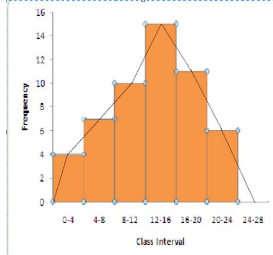 Steps for construction:
(i) Draw a histogram for the given data.
(ii) Mark the mid-point at the top of each rectangle of the histogram drawn.
(iii) Also, mark the mid-point of the immediately lower class-interval and mid-point of the immediately higher class-interval.
(iv) Lastly, join the consecutive mid-points marked by straight lines to obtain the required frequency polygon.
Steps for construction:
(i) Draw a histogram for the given data.
(ii) Mark the mid-point at the top of each rectangle of the histogram drawn.
(iii) Also, mark the mid-point of the immediately lower class-interval and mid-point of the immediately higher class-interval.
(iv) Lastly, join the consecutive mid-points marked by straight lines to obtain the required frequency polygon.
2. Construct a combined histogram and frequency polygon for the following frequency distribution:
| Class Intervals | 10 – 20 | 20 – 30 | 30 – 40 | 40 – 50 | 50 – 60 |
| Frequency | 3 | 5 | 6 | 4 | 2 |
Solution:
The combined histogram and frequency polygon for the given data is shown below: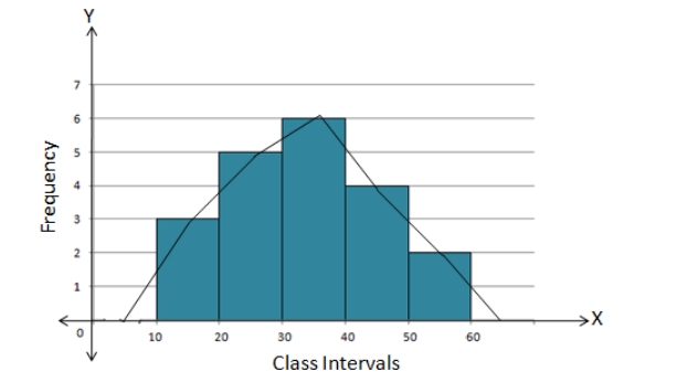 Steps for construction:
(i) Draw a histogram for the given data.
(ii) Mark the mid-point at the top of each rectangle of the histogram drawn.
(iii) Also, mark the mid-point of the immediately lower class-interval and mid-point of the immediately higher class-interval.
(iv) Lastly, join the consecutive mid-points marked by straight lines to obtain the required frequency polygon.
Steps for construction:
(i) Draw a histogram for the given data.
(ii) Mark the mid-point at the top of each rectangle of the histogram drawn.
(iii) Also, mark the mid-point of the immediately lower class-interval and mid-point of the immediately higher class-interval.
(iv) Lastly, join the consecutive mid-points marked by straight lines to obtain the required frequency polygon.
3. Construct a frequency polygon for the following data:
| Class-Intervals | 10 – 14 | 15 – 19 | 20 – 24 | 25 – 29 | 30 – 34 |
| Frequency | 5 | 8 | 12 | 9 | 4 |
Solution:
As the class intervals are inclusive, let’s first convert them into the exclusive form.| Class-Interval | Frequency |
| 9.5 – 14.5 | 5 |
| 14.5 – 19.5 | 8 |
| 19.5 – 24.5 | 12 |
| 24.5 – 29.5 | 9 |
| 29.5 – 34.5 | 4 |
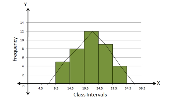 Steps for construction:
(i) Draw a histogram for the given data.
(ii) Mark the mid-point at the top of each rectangle of the histogram drawn.
(iii) Also, mark the mid-point of the immediately lower class-interval and mid-point of the immediately higher class-interval.
(iv) Lastly, join the consecutive mid-points marked by straight lines to obtain the required frequency polygon.
Steps for construction:
(i) Draw a histogram for the given data.
(ii) Mark the mid-point at the top of each rectangle of the histogram drawn.
(iii) Also, mark the mid-point of the immediately lower class-interval and mid-point of the immediately higher class-interval.
(iv) Lastly, join the consecutive mid-points marked by straight lines to obtain the required frequency polygon.
4. The daily wages in a factory are distributed as follows:
| Daily wages (in Rs.) | 125 – 175 | 175 – 225 | 225 – 275 | 275 – 325 | 325 – 375 |
| Number of workers | 4 | 20 | 22 | 10 | 6 |
Draw a frequency polygon for this distribution.
Solution:
The frequency polygon for the given data is shown as below Steps for construction: (i) Draw a histogram for the given data. (ii) Mark the mid-point at the top of each rectangle of the histogram drawn. (iii) Also, mark the mid-point of the immediately lower class-interval and mid-point of the immediately higher class-interval. (iv) Lastly, join the consecutive mid-points marked by straight lines to obtain the required frequency polygon.5. (i) Draw frequency polygons for each of the following frequency distribution:
(a) using histogram
(b) without using histogram
| C.I | 10 – 30 | 30 – 50 | 50 – 70 | 70 – 90 | 90 – 110 | 110 – 130 | 130 – 150 |
| ƒ | 4 | 7 | 5 | 9 | 5 | 6 | 4 |
Solution:
(a) Using Histogram:| Class Interval | Frequency |
| 10 – 30 | 4 |
| 30 – 50 | 7 |
| 50 – 70 | 5 |
| 70 – 90 | 9 |
| 90 – 110 | 5 |
| 110 – 130 | 6 |
| 130 – 150 | 4 |
The frequency polygon for the given data is shown as below
Steps for construction: (i) Draw a histogram for the given data. (ii) Mark the mid-point at the top of each rectangle of the histogram drawn. (iii) Also, mark the mid-point of the immediately lower class-interval and mid-point of the immediately higher class-interval. (iv) Lastly, join the consecutive mid-points marked by straight lines to obtain the required frequency polygon. (b) Without using Histogram: Steps for construction: (i) Find the class mark (mid-value) of each given class-interval. Using, Class mark = mid-value = (Upper limit + Lower limit)/2 (ii) On a graph paper, mark class marks along X-axis and frequencies along Y-axis. (iii) On this graph paper, mark points taking values of class-marks along X-axis and the values of their corresponding frequencies along Y-axis. (iv) Draw line segments joining the consecutive points marked in step (3) above.| C.I. | Class mark | Frequency |
| 0 – 10 | 0 | 0 |
| 10 – 30 | 20 | 4 |
| 30 – 50 | 40 | 7 |
| 50 – 70 | 60 | 5 |
| 70 – 90 | 80 | 9 |
| 90 – 110 | 100 | 5 |
| 110 – 130 | 120 | 6 |
| 130 – 150 | 140 | 4 |
| 150 – 170 | 160 | 0 |
5. (ii) Draw frequency polygons for each of the following frequency distribution:
(a) using histogram
(b) without using histogram
| C.I | 5 – 15 | 15 – 25 | 25 – 35 | 35 – 45 | 45 – 55 | 55 – 65 |
| ƒ | 8 | 16 | 18 | 14 | 8 | 2 |
Solution:
(a) Using Histogram:| C.I. | Frequency |
| 5 – 15 | 8 |
| 15 – 25 | 16 |
| 25 – 35 | 18 |
| 35 – 45 | 14 |
| 45 – 55 | 8 |
| 55 – 65 | 2 |
| C.I. | Class mark | Frequency |
| 5 – 15 | 0 | 0 |
| 5 – 15 | 10 | 8 |
| 15 – 25 | 20 | 16 |
| 25 – 35 | 30 | 18 |
| 35 – 45 | 40 | 14 |
| 45 – 55 | 50 | 8 |
| 55 – 65 | 60 | 2 |
| 65 – 75 | 70 | 0 |
Benefits of ICSE Class 9 Maths Selina Solutions Chapter 18
ICSE Class 9 Maths Selina Solutions for Chapter 18 on Statistics provide several key benefits for students, enhancing their understanding and proficiency in the subject. Here’s a concise overview: 1. Conceptual UnderstandingClear Explanations: Solutions offer detailed, step-by-step explanations for statistical concepts such as mean, median, mode, and measures of dispersion. This helps in building a strong foundational understanding.
Visual Aids: The use of graphs and charts in the solutions aids in visualizing data, making it easier to grasp statistical concepts.
2. Enhanced Problem-Solving SkillsDiverse Problems: Exposure to various types of problems helps students practice different techniques for analyzing and interpreting statistical data.
Methodical Approach: Solutions demonstrate systematic methods to solve problems, reinforcing correct procedures and improving analytical skills.
3. Effective Exam PreparationICSE Syllabus Alignment: Solutions are aligned with the ICSE curriculum, ensuring students are well-prepared for their exams with relevant examples and question types.
Familiarity with Exam Patterns: Practicing with these solutions helps students become familiar with common exam questions and formats, aiding in better time management and exam performance.
4. Self-Study and RevisionIndependent Learning: Provides a valuable resource for students to study and revise statistical concepts on their own, enhancing their ability to work independently.
Error Correction: Students can identify and correct mistakes by comparing their solutions with the provided ones, leading to improved accuracy and understanding.
Here at Physics Wallah we provide the Best CLASS 9 ONLINE COACHING to ease your exam preparation. Our class 9 online courses are taught by well-known instructors. We attempt to strengthen conceptual understanding and foster problem-solving abilities.ICSE Class 9 Maths Selina Solutions Chapter 18 FAQs
What is the syllabus of class 9 ICSE maths?
What is a rational and irrational number Class 9?
Is 0 a real number?
Is ICSE checking strict?