

CBSE Class 11 Maths Notes Chapter 15 Statistics

CBSE Class 11 Maths Notes Chapter 15: In CBSE Class 11 Maths Chapter 15, you'll learn about Statistics. Statistics is all about gathering, organizing, analyzing, and presenting data. You'll discover how to find the average value of a set of numbers, which is called the mean, as well as other measures like median and mode.
These help you understand what's typical or common in a group of data. You'll also learn about range, variance, and standard deviation, which tell you how spread out the data is. By mastering mathematical reasoning, you’ll improve your problem-solving skills and understand math concepts better.CBSE Class 11 Maths Notes Chapter 15 PDF
You can find the CBSE Class 11 Maths Notes Chapter 14 on Statistics in PDF format through the link provided below. By using this PDF, you can learn how to analyze math statements, recognize patterns, and make logical conclusions, which will improve your problem-solving skills in math.CBSE Class 11 Maths Notes Chapter 15 PDF
CBSE Class 11 Maths Notes Chapter 15 Statistics
Statistics
Statistics is a branch of mathematics that deals with the collection, organization, analysis, interpretation, and presentation of data. It provides methods for summarizing and making inferences from large sets of numerical information, aiding decision-making in various fields such as science, business, economics, and social sciences.Limit of the Class
In statistics, when data is organized into groups or classes, each class has two limits: the lower limit and the upper limit. These limits define the range of values included in each class. The upper limit is the highest value in the class, while the lower limit is the lowest value.Class Interval
The class interval, also known as the class width, is the difference between the upper and lower limits of a class. It determines the range of values that fall within each class and is essential for organizing data into meaningful groups for analysis.Primary and Secondary Data
Primary data refers to information collected directly from original sources by the researcher or investigator. This data is firsthand and specific to the research purpose. On the other hand, secondary data is data that has been collected, processed, and published by others. It may include sources such as books, journals, government publications, and online databases.Variable or Variate
In statistics, a variable or variate is any characteristic, number, or quantity that can vary or take different values in different situations. Variables can be classified as independent or dependent, qualitative or quantitative, discrete or continuous, among other categories.Frequency
Frequency refers to the number of times a particular observation or value occurs in a dataset. It provides information about the distribution or pattern of data and helps identify common or rare occurrences within the dataset.Discrete Frequency Distribution
Discrete frequency distribution is a method of organizing and summarizing data that consists of distinct, separate values or categories. Each value in the dataset is assigned a frequency based on how often it occurs. This type of distribution is commonly used for counting occurrences of categorical or countable variables.Continuous Frequency Distribution
Continuous frequency distribution is used when data falls into ranges or intervals rather than individual values. It involves grouping data into intervals of continuous values and assigning frequencies to each interval. This type of distribution is suitable for measuring continuous variables, such as height, weight, or temperature.Cumulative Frequency Distribution
Cumulative frequency distribution provides a cumulative count of frequencies up to a certain point or class in a dataset. It involves adding the frequencies of each class successively to obtain cumulative totals. This type of distribution helps analyze the cumulative distribution of data and identify trends or patterns across different intervals or classes.Graphical Representation Of Frequency Distribution
Histogram
A histogram is a graphical representation of the frequency distribution of a dataset. It is constructed by marking the class intervals of the data on the x-axis and their corresponding frequencies on the y-axis. Each class interval is represented by an erected rectangle, where the width of the rectangle is proportional to the width of the class interval, and the height is proportional to the frequency of that interval. In the case of unequal class intervals, the height of the rectangles is adjusted to maintain proportionality. Specifically, the height is determined by the ratio of the frequency of each class interval to the width of that interval. This ensures that the area of each rectangle accurately reflects the frequency of the corresponding class interval. Histograms provide a visual depiction of the distribution of data, allowing for easy interpretation and analysis. They are particularly useful for identifying patterns, trends, and outliers within the dataset. The example below illustrates a sample histogram: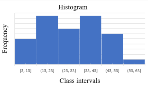
Bar diagram
In bar diagrams, only the length of the bars or rectangles is considered. The data is first divided into different classes, and then these classes are marked with equal widths on the x-axis. Corresponding frequencies are then marked on the y-axis, with each frequency being proportional to the length of the corresponding bar. Bar diagrams provide a visual representation of the distribution of data, making it easier to compare different categories or groups. They are commonly used to display categorical data and are effective for showing relative frequencies or counts within each category. Below is an example illustrating a bar diagram: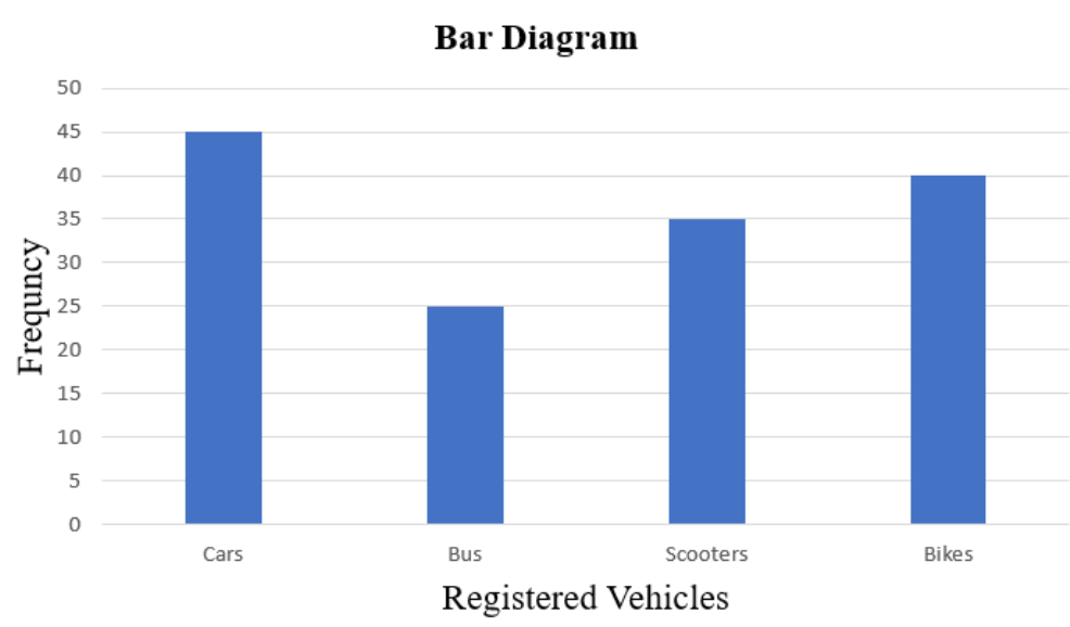
Pie diagrams
Pie charts are commonly used to represent relative frequency distributions, where a circle is divided into sectors corresponding to the number of classes or categories. The area of each sector is proportional to the frequency of that class or category. These charts provide a visual representation of how the whole is divided into parts. To draw the required sectors in a pie chart, we calculate the central angle for each class using the formula: Central angle=Frequency×360∘Total frequency This formula helps in proportionately dividing the angles to represent the relative frequencies. Pie charts are effective for presenting data with a limited number of categories and can quickly convey the proportion of each category relative to the whole. Below is an example illustrating a pie chart: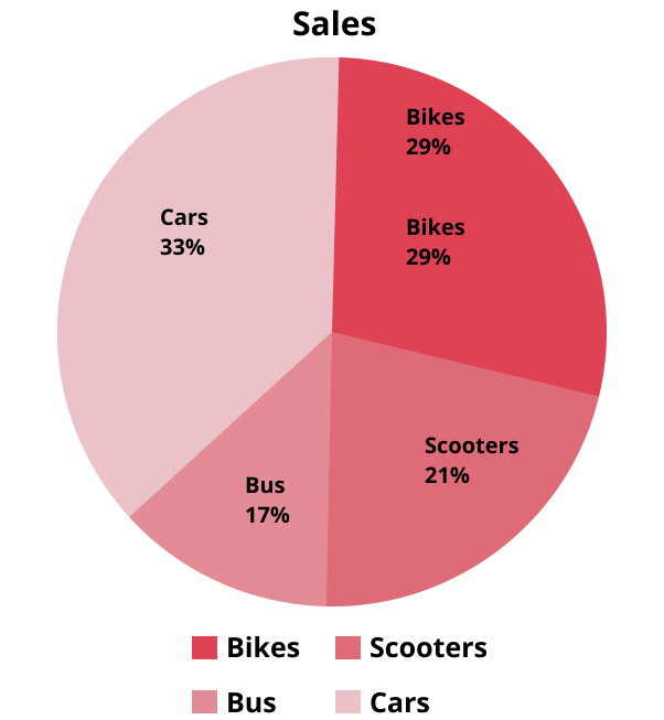
Frequency Polygon
To create a frequency polygon for an ungrouped frequency distribution, we first plot the variate values on the x-axis and the corresponding frequencies on the y-axis. Then, we locate the midpoints of each bar representing the variate values and connect these midpoints using straight lines. This process helps to visualize the trend of the data distribution. Here's an example illustrating the construction of a frequency polygon: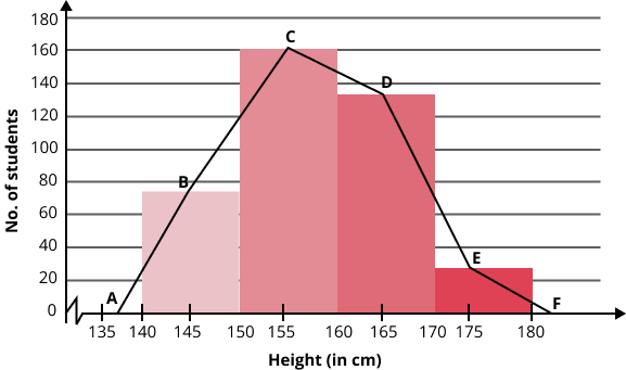
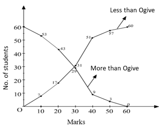
Cumulative frequency curve (Ogive)
To construct a cumulative frequency curve, also known as an ogive, we begin by preparing a cumulative frequency table based on the given data. Then, we plot the cumulative frequencies against either the upper or lower limits of the corresponding class intervals. Next, we connect the plotted points to form a smooth curve. There are two main methods for drawing an ogive:Less than method : In this method, we plot the upper limits of the class intervals on the x-axis and the corresponding cumulative frequencies (less than cumulative frequencies) on the y-axis. We then connect these points with smooth curves to form the less than ogive, which is also known as a falling curve.
More than method : In this method, we plot the lower limits of the class intervals on the x-axis and the corresponding cumulative frequencies (more than cumulative frequencies) on the y-axis. Similar to the less than method, we connect these points with smooth curves to form the more than ogive, which is also known as a rising curve.
Measures Of Central Tendency
Measures of central tendency provide valuable insights into the central value of a dataset. The five key measures of central tendency are:Arithmetic Mean : It's the average of a set of numbers. There are different formulas depending on the nature of the data:
- For unclassified data: Sum of all values divided by the total number of values.
- For frequency distribution: Sum of (value × frequency) divided by the sum of frequencies.
- For classified data: Sum of (class mark × frequency) divided by the sum of frequencies.
- Using the step deviation method for classified data.
- Combined mean for multiple groups of observations.
- Weighted arithmetic mean, which considers weights assigned to each value.
Median : The middle value of a dataset when arranged in ascending or descending order. If there is an even number of values, the median is the average of the two middle numbers.
- Mode : The most frequently occurring value in a dataset.
- Geometric Mean : The nth root of the product of n values.
- Harmonic Mean : The reciprocal of the arithmetic mean of the reciprocals of a set of numbers.
Properties Of Arithmetic Mean
a) Arithmetic Means : These averages remain unchanged regardless of shifting the entire data set by a constant value (change of origin) or multiplying each data point by a constant value (change of scale). b) Sum of Deviations : The total sum of deviations of individual values from the arithmetic mean of a dataset is always zero. This property holds true for any set of data. c) Minimum Sum of Squares : When considering the sum of squares of deviations from the mean, this sum is at its minimum value when calculated about the mean. This means that the arithmetic mean is the measure around which the deviations are minimized. d) Geometric Mean : It is a measure of central tendency specifically used for data sets with values that multiply together. It's calculated as the nth root of the product of n values. e) Harmonic Mean : This measure is used for sets of numbers where rates are involved, such as speed or time. It's calculated as the reciprocal of the arithmetic mean of the reciprocals of the data set. f) Median : The middle value in a sorted dataset, unaffected by extreme values, making it a robust measure of central tendency. g) Quartiles : These are values that divide the data set into four equal parts, useful for understanding the distribution of data across the range. h) Mode : It's the value that appears most frequently in a dataset. For grouped data, the mode is the midpoint of the modal class, the class with the highest frequency. i) Relationship Between Mean, Median, and Mode : There exists a relationship between these three measures. For example, the mode is approximately three times the median minus two times the mean. This relationship can provide insights into the distribution of data.Symmetrical And Skew Distribution
a) Symmetric Distribution : In a symmetric distribution, the frequencies are evenly distributed around the mode, resulting in a bell-shaped curve. In such cases, the arithmetic mean, median, and mode are all equal. b) Positive Skewness : This occurs when the distribution is skewed to the right. The arithmetic mean is greater than the median, which in turn is greater than the mode. c) Negative Skewness : In this scenario, the distribution is skewed to the left. Here, the arithmetic mean is less than the median, which is less than the mode.Measures of Dispersion:
- Range : This is the difference between the highest and lowest values in the dataset. It provides a simple measure of spread but is sensitive to outliers.
- Quartiles and Quartile Deviation : Quartiles divide the data into four equal parts, while quartile deviation measures the spread around the median.
- Mean Deviation : This is the average of the absolute deviations from the mean, median, or mode. It provides a measure of variability but is less sensitive to outliers than the range.
- Standard Deviation and Variance : Standard deviation measures the average deviation from the mean, while variance is the square of the standard deviation. These are widely used measures of spread and are sensitive to outliers.
Analysis of Frequency Distributions:
- Coefficient of Variation : This measure compares the standard deviation to the mean, providing a relative measure of variability that is independent of the units of measurement.
- Consistency and Variability : A lower coefficient of variation indicates greater consistency, while a higher standard deviation suggests greater variability.
- Comparing Distributions : When comparing two distributions with equal means, the one with a higher standard deviation is considered more variable, while the one with a lower standard deviation is more consistent.
Benefits of CBSE Class 11 Maths Notes Chapter 15 Statistics
Comprehensive Coverage : The notes cover all essential topics and concepts included in the CBSE Class 11 Mathematics syllabus for Statistics. This ensures that students have access to all the necessary information required to understand the subject thoroughly.
Clarity and Simplification : The notes are written in simple language, making it easier for students to grasp complex statistical concepts. They provide clear explanations, examples, and illustrations to aid in better understanding.
Structured Format : The notes are well-organized, following the sequence of topics as per the curriculum. This structured format helps students to follow along and locate specific information quickly when revising or studying.
Accessibility : The notes are available in PDF format, making them easily accessible to students anytime, anywhere. They can be downloaded and stored on digital devices or printed out for offline use, ensuring flexibility and convenience.
Preparation for Exams : By studying these notes, students can enhance their exam preparation and performance. They provide a detailed overview of the subject, helping students to revise effectively and score well in exams.
CBSE Class 11 Maths Notes Chapter 15 FAQs
What is Statistics?
What are the measures of central tendency?
What is the difference between mean, median, and mode?
What is the range of a data set?
What is standard deviation?