Potential
Electrostatics of Class 12
POTENTIAL
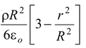
The motion of a particle with positive charge q in a uniform electric field is analogous to the motion of a particle of mass m, in the uniform gravitational field near the surface of earth. To move a particle against the field requires work by an external agent.
|
If the external force is equal and opposite to the force due to the field, the kinetic energy of the particle will not change. In this case, all the external work is stored as potential energy in the system. Wext = +ΔU = Uf − Ui(1.9) where Uf and Ui are the final and initial potential energies. The gravitational potential energy function near the surface of the earth is Ug = mgy. |
|
One can obtain a function that does not depend on m by defining the gravitational potential as the potential energy per unit mass: Vg = Ug/m = gy. The SI unit of Vg is J/kg. The gravitational potential at a point is the external work needed to lift a unit mass from the zero level of potential (y = 0) to the given height, without a change in speed.
When a charge q moves between two points in an electrostatic field, the change in electric potential, ΔV is defined as the change in electrostatic potential energy per unit charge.
ΔV = ΔU/q (1.10)
The SI unit of electric potential is the volt (V).
Note that 1V = 1 J/C
The quantity ΔV depends only on the field set up by the source charges, not on the test charge. Once the potential difference between two points is known, the external work needed to move a charge q, with no change in its speed, may be found from equation (1.10).
Wext = qΔV = q (Vf − Vi)(1.11)
The sign of this work depends on the sign of q and the relative magnitudes of Vi and Vf.
If Wext > 0, work is done by the external agent on the charge.
If Wext < 0 , work is done on the external agent by the field. In the latter case, in order to keep the speed constant, the external force acts opposite to the displacement of the charge.
The potential at a point is the external work needed to bring a positive unit charge, at constant speed, from the position of zero potential to the given point. Conventionally, the point of zero potential is taken at infinity.
Relationship between E and V
We know that
ΔV = Wext/q
Now Wext = 
Since the external force is equal and opposite to the electrostatic force
Therefore, 
orWext = −
|
The Fig. (1.14) shows a curved path in a non−uniform field. The potential difference between the points A and B is given by
VB − VA = Since the electrostatic field is conservative the value of this line integral depends only on the end points A and B, not on the path taken. The equation (1.12) can be used to find the potential function if electric field function is given. Let us see, how to obtain an expression for electric field if potential function is known? |
|

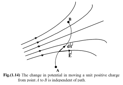
An infinitesimal change in potential associated with the displacement ds is given by
dV = −E .ds = −Eds cosθ
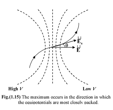
Since Es = E cosθ is the component of E along ds, the above equation may be written as dV = −Es ds, from which we infer that
Es = −dV/dz]s(1.13)
Since the direction of ds is arbitrary, equation (1.13) may be interpreted as follows:
Any component of E may be found from the rate of V with distance in the chosen direction. There will be one direction for which this rate of change is a maximum. The magnitude of E is given by this maximum value of the spatial derivative: that is E = −(dV/ds)max. As figure (1.15) shows, the maximum occurs in the direction in which the equipotentials are most closely spaced.
|
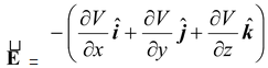
In rectangular components the electric field is E = Exi + Eyj + Ezk and an infinitesimal displacement is ds = dxi + dyj + dzk. Thus, dV = −E. ds = −(Exdx + Eydy + Ezdz) For a displacement in the x direction, dy = dz = 0 and so dV = −Exdx. Therefore, Ex = (-dV/dx) A derivative in which all variables except one are held constant is called partial derivative and is written with a ∂ instead of d. The electric field is therefore |
|
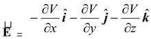 (1.14)
The right side of equation (1.14) is called the gradient of V. There are no new rules of differentiation to learn, as the following example illustrates.
In polar coordinates
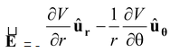 (1.15)
where ur and uθ are the unit vectors in the radial and tangential directions.
Example: 1.7
A hypothetical potential function has the following form
V(x,y,z) = 2x3y − 3xy2z + 5yz3
Obtain an expression for electric field
Solution
Using equation (1.14)
Here ∂V/∂x = 6x2y − 3y2z; ∂V/∂y = 2x3 − 6xyz + 5z2; ∂V/∂z = −3xy2 + 15yz2
Thus, E = (−6x2y + 3y2z)i + (−2x3 + 6xyz − 5z3) j + (3xy2 − 15yz2) k
Potential of a point charge
Let us see how the potential varies in the vicinity of a point charge Q. The electric field is

Since E is radially outward and ds is radially inward therefore E.ds = −Eds
and also, ds = -dr, therefore –Eds = Edr.
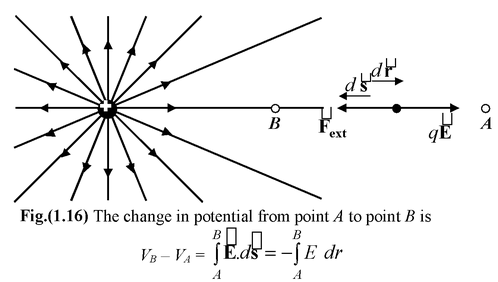
Thus equation (1.12) the change in potential moving from A to B may be reduced as
VB − VA = 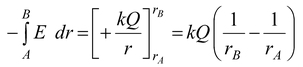
If we choose V = 0 at r = ∞, this implies that the point A shifts to the infinity.
V = kQ/r (1.16)
Potential of a system of Point Charges
When several point charges are present, the total potential at same point is given by the algebraic sum of the potentials due to all the charges.
V =  (1.17)
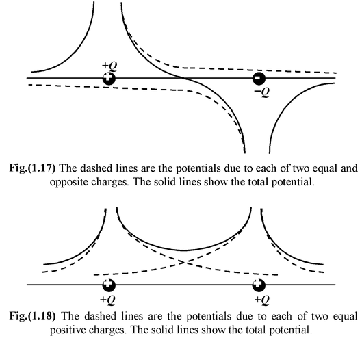
The Fig. (1.17) shows the potential of two equal and opposite point charges. The dotted curves are the individual potential functions whereas the solid curve is the total potential function that would be encountered when the two charges are brought closer. Notice that at the mid−point V = 0 but E ≠ 0. Fig. (1.18) shows the total potential due to two equal positive point charges. Notice that at the mid−point E = 0 but V ≠ 0.
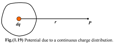
Potential Due to a Continuous Charge Distribution
The potential due to a continuous charge distribution may be obtained in two ways.
First method
Find the potential at the given point (see fig. (1.19)) due to an infinitesimally small point charge dq.
|
That is dV = kdq/r Integrate this expression over the whole charge distribution V = k ∫dq/r (1.18) |
|
Second method
If E is already known − for example, Gauss law − then potential may be obtained from equation
VB − VA = 
Example: 1.8
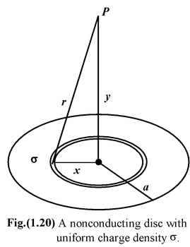
A nonconducting disc of radius a has a uniform surface charge density σ C/m2. What is the potential at a point on the axis of the disc at a distance y from its center ?
Solution
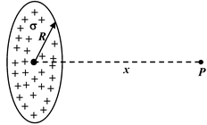
The symmetry of the disc tells us that the appropriate choice of element is a ring of radius x and thickness dx, as shown in the figure (1.20). All points on this ring are at the same distance, r = (x2 + y2)1/2, from the point P. The charge on the ring is
dq = σ dA = σ(2π xdx) and so the potential due to the ring is
dV = 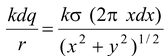
Since the potential is a scalar, there are no components to worry about.
Note that there is only one variable x, in this expression, the distance y is fixed. The potential due to the whole disk is the integral of the above expression.
V = 2πkσ 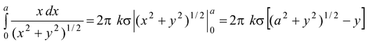
|
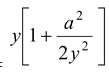
Using binomial theorem [(1 + z)n ≈ 1 + nz] for small z to expand the first term : when y >> a, a/y <<1. Then
(a2 + y2)1/2 = y
= Substituting this into the expression for V we find V = kQ/y where Q =σπa2 is the total charge on the disc. At large distances, the potential due to the disc is the same as that of a point charge Q. |
|

Equipotential Lines
There is another way of representing the electrostatic fields : the method of equipotential lines or surfaces. It is a locus of points all of which have the same potential.
If the source of the field is a point charge, then one can easily see from equation (1.16) that the equipotential surfaces will constitute a family of concentric spheres with their centre at the point where the charge is located.
|
In the figure (1.21) the equipotentials are drawn as dashed circles and the solid radial lines represent the fields lines. Near the charge the potential changes rapidly with distance, so the equipotentials are close together. The field lines are always normal to the equipotentials and point toward lower values of potential. The field is strong where the equipotentials are closely spaced. |
|
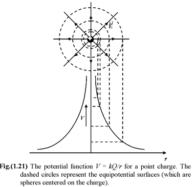
Table 1.2 Electric Potential V due to Various Charge Distribution
|
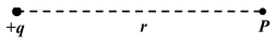
1.Isolated Charge
|
V = |
|
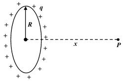
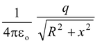
2.A Ring of Charge
|
V = |
|
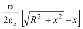
3.A Disc of Charge
|
V = |
|
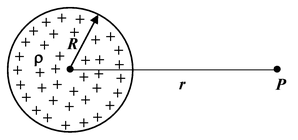
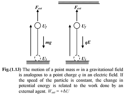
4.A sphere of Charge
|
Inside 0 ≤ r ≤ R
V = Outside r ≥ R
V = where ρ is the volume charge density. |